SQL Window Functions in Production: What the Tutorials Don't Tell You

This article is written for engineers who already know what a JOIN is and want to understand window functions at the level needed to use them confidently in production systems — not just pass a technical screen.

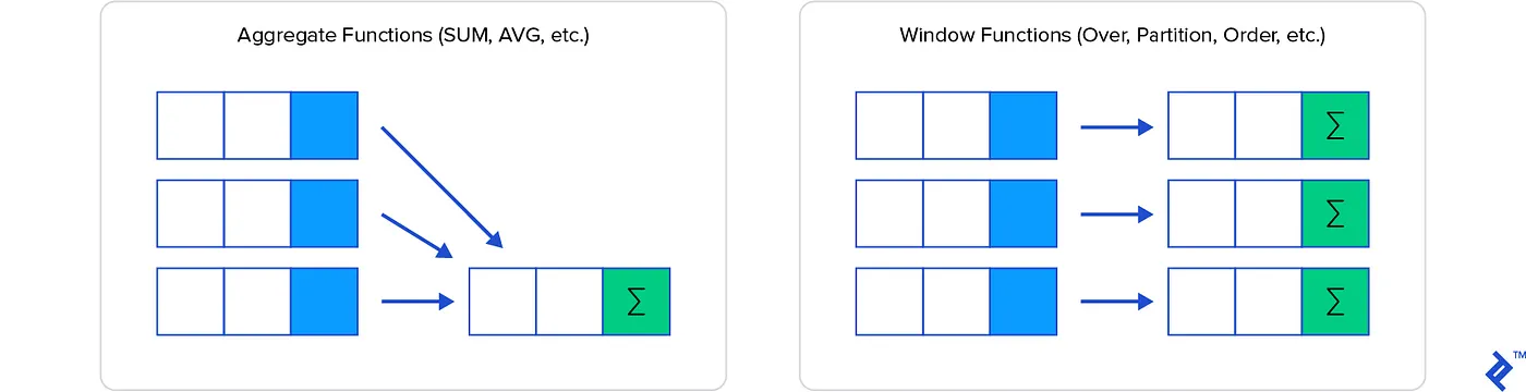
Why Aggregates Aren’t Enough

A standard aggregate function collapses rows. GROUP BY rep_name turns ten sales rows into one summary row per rep. That’s often exactly what you want — but the moment your query needs both the detail row and a summary statistic computed across a group, you’re in trouble.

The traditional workarounds are well-known and uniformly painful:

Correlated subqueries recompute a full scan for every row in the outer query. On a 10,000-row result set, that’s 10,000 separate subquery executions — each one potentially doing a sequential scan or index lookup.

-- This runs the subquery once per row in sales
SELECT
    s1.sale_id,
    s1.rep_name,
    s1.sale_amount,
    (SELECT SUM(s2.sale_amount)
     FROM sales s2
     WHERE s2.rep_name = s1.rep_name
       AND s2.sale_month <= s1.sale_month) AS running_total
FROM sales s1;

On a table of 500k rows, this query can run for minutes on a well-indexed Postgres instance. With window functions, the planner materializes the relevant partition once and streams through it — the difference can be an order of magnitude.

CTEs with self-joins are structurally cleaner but carry their own costs. Pre-Postgres 12, CTEs were optimization fences — the planner couldn’t push predicates through them. Even today, a self-join on a large CTE often means materializing the intermediate result twice.

Application-side aggregation — pulling raw rows and computing running totals in Python or Go — shifts CPU load off the database but introduces network transfer overhead and makes the computation harder to optimize, audit, or cache.

The Execution Model

Before writing a window function in production code, it’s worth understanding what the query planner actually does with it.

When PostgreSQL encounters a window function, it inserts a WindowAgg node into the query plan. That node:

1. Sorts the input relation by the PARTITION BY and ORDER BY keys
2. Streams through sorted rows, maintaining state per partition
3. Emits one output row per input row — preserving cardinality

The sort step is the expensive part. For small datasets or queries with an index that already provides the required ordering, this is cheap. For large datasets with no supporting index, you’re paying for an explicit sort — which means memory allocation for the sort buffer, and a potential spill to disk if work_mem isn’t large enough.

-- EXPLAIN ANALYZE output for a window function on an unindexed column
-- Sort  (cost=47823.12..49323.12 rows=600000 width=48)
--   Sort Key: rep_name, sale_month
--   Sort Method: external merge  Disk: 18432kB   <-- spilling to disk
--   ->  Seq Scan on sales  (cost=0.00..9637.00 rows=600000 width=48)

A disk spill is often the difference between a sub-second analytics query and one that saturates your I/O. The fix is usually composite index creation or increasing work_mem for the session — but understand the tradeoff: work_mem is per sort operation per connection, so bumping it globally on a busy server can cause OOM conditions.

Window Function Anatomy

The OVER clause is where the semantics live. It has three optional components:

function_name(args) OVER (
    PARTITION BY col1, col2   -- defines independent groups
    ORDER BY col3             -- defines ordering within each partition
    ROWS BETWEEN 2 PRECEDING AND CURRENT ROW  -- defines the frame
)

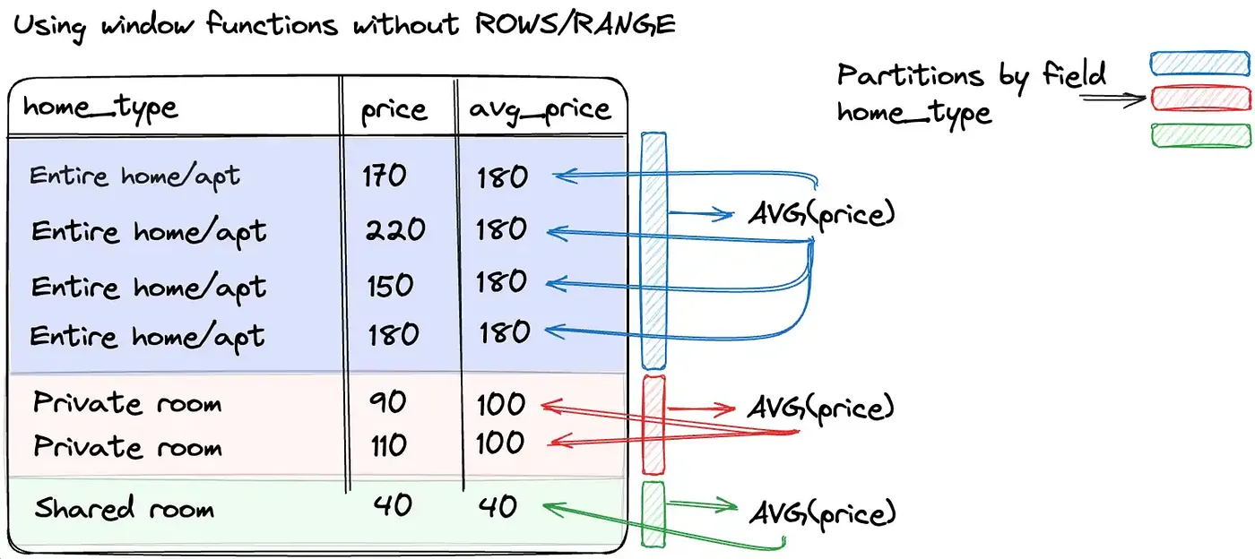
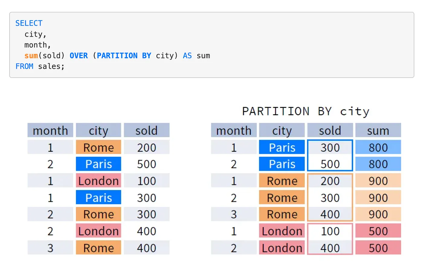
PARTITION BY — Creates independent windows. Each partition is processed separately; no state bleeds across partition boundaries. Functionally similar to GROUP BY but without row collapsing.

ORDER BY — Required for any function that depends on row position (LAG, LEAD, RANK, NTILE, running aggregates). Without it, the frame is undefined and functions like SUM(...) OVER (PARTITION BY ...) compute the total for the entire partition for every row — which is sometimes what you want, sometimes a silent correctness bug.

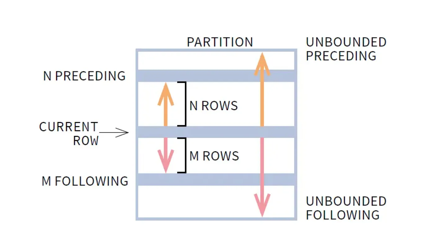
Frame specification — The most underused and most powerful part. Without an explicit frame, ROWS BETWEEN UNBOUNDED PRECEDING AND CURRENT ROW is the default when ORDER BY is present. This gives you a running aggregate. Specify ROWS BETWEEN 6 PRECEDING AND CURRENT ROW and you get a 7-row rolling window. Specify ROWS BETWEEN UNBOUNDED PRECEDING AND UNBOUNDED FOLLOWING and you get the full-partition aggregate on every row.

A Real Production Query

The canonical use case: a sales reporting system where the analytics team wants rep-level running totals, monthly rankings, and period-over-period deltas — all in one pass.

SELECT
    sale_id,
    rep_name,
    sale_month,
    sale_amount,
    -- Running total per rep, reset each calendar year
    SUM(sale_amount) OVER (
        PARTITION BY rep_name, EXTRACT(year FROM sale_month)
        ORDER BY sale_month
        ROWS BETWEEN UNBOUNDED PRECEDING AND CURRENT ROW
    ) AS ytd_total,
    -- Rank within month, dense so no gaps in ranking
    DENSE_RANK() OVER (
        PARTITION BY sale_month
        ORDER BY sale_amount DESC
    ) AS monthly_rank,
    -- Month-over-month delta per rep
    sale_amount - LAG(sale_amount, 1, 0) OVER (
        PARTITION BY rep_name
        ORDER BY sale_month
    ) AS mom_delta,
    -- 3-month rolling average
    AVG(sale_amount) OVER (
        PARTITION BY rep_name
        ORDER BY sale_month
        ROWS BETWEEN 2 PRECEDING AND CURRENT ROW
    ) AS rolling_3mo_avg
FROM sales
WHERE sale_month >= '2024-01-01'
ORDER BY sale_month, rep_name;

This is four window functions across the same base table — and with a proper composite index on (rep_name, sale_month), PostgreSQL can satisfy all of them with a single sort pass using window function optimization (multiple windows sharing the same sort key are executed together).

The Ranking Functions: Correctness Details

Three functions, one job, three different semantics — and choosing wrong produces silent data errors.

ROW_NUMBER() — Assigns a strictly unique sequential integer to every row within the partition. Ties are broken arbitrarily (or by adding more ORDER BY columns). Use this when you need exactly N rows — for example, “the most recent 3 orders per customer.”

RANK() — Assigns the same rank to tied rows, then skips ahead. Ranks 1, 2, 2, 4. Use when the absolute position matters — a sales rep ranked 4th actually lost to three others, including two who tied for 2nd.

DENSE_RANK() — Assigns the same rank to tied rows, no skipping. Ranks 1, 2, 2, 3. Use when the rank itself is a meaningful label (e.g., “top 3 performers”) and gaps in the sequence would be confusing.

The failure mode: using ROW_NUMBER() for a “top N per group” query when you actually want all tied records in the Nth position. You’ll silently exclude valid results.

-- WRONG: may exclude tied reps at the cutoff
SELECT * FROM (
    SELECT *, ROW_NUMBER() OVER (ORDER BY sale_amount DESC) AS rn FROM sales
) WHERE rn <= 3;

-- RIGHT: includes all reps tied at position 3
SELECT * FROM (
    SELECT *, DENSE_RANK() OVER (ORDER BY sale_amount DESC) AS dr FROM sales
) WHERE dr <= 3;

How This Applies to Distributed Systems

Window functions are typically a database-layer concern, but the concepts map directly to distributed stream processing.

Partitioning = Sharding key selection. PARTITION BY customer_id in SQL maps to partitioning a Kafka topic by customer_id in a streaming pipeline. Both ensure that all events for a given entity land in the same processing context — a prerequisite for correctness in stateful computations.

Ordered frames = Watermarks. The ORDER BY sale_month inside a window defines what “position” means relative to the current row. In systems like Apache Flink or Spark Structured Streaming, watermarks play the same role: they define how far behind the stream is allowed to fall before the window closes and results are emitted. Get the watermark wrong and you either drop late events or never emit results.

Running aggregates = Accumulator state. A SUM(...) OVER (ORDER BY ts) is structurally identical to a Flink ProcessFunction that maintains a running sum in managed state. The difference is fault tolerance: the database handles this atomically within a transaction; a stream processor needs explicit checkpointing to recover without replay from scratch.

LAG / LEAD = Event sequencing. In fraud detection, “the previous transaction for this card” is a LAG computation. In a distributed system, this requires either total ordering within a partition or a secondary index lookup — which has latency implications that an in-database LAG avoids entirely.

Production Failure Case: Partition Skew Under Load

Here’s a scenario that played out on a reporting system running against a multi-tenant SaaS database.

Setup: A nightly job generates per-tenant analytics using window functions. The query partitions by tenant_id and orders by created_at. The team has ~2,000 tenants. Most have a few hundred rows. Three enterprise tenants have 4-8 million rows each.

The query:

SELECT
    tenant_id,
    user_id,
    event_at,
    COUNT(*) OVER (PARTITION BY tenant_id ORDER BY event_at
                   ROWS BETWEEN UNBOUNDED PRECEDING AND CURRENT ROW) AS session_event_count
FROM events
WHERE event_at >= NOW() - INTERVAL '30 days';

What happened: The query ran fine in staging (small dataset). In production, the three large tenants caused the WindowAgg sort to spill to disk — multiple times, for partitions with millions of rows. The job that was expected to complete in 4 minutes ran for 47 minutes. It held open a long transaction, which bloated the replica’s replication lag to 12 minutes. The monitoring dashboard, which read from the replica, started showing stale data. An oncall was paged for a “data outage” that was actually a query planning failure.

Debugging path: EXPLAIN (ANALYZE, BUFFERS) revealed the disk spills. pg_stat_activity showed the long-running query. The fix was two-part: add a composite index on (tenant_id, event_at) to eliminate the sort, and process large-tenant partitions in a separate query with elevated work_mem via SET LOCAL.

The lesson: Window function performance is partition-dependent. A query that runs in 200ms on 98% of your data can degrade catastrophically on the remaining 2% if partition sizes are skewed. Always EXPLAIN ANALYZE against production-representative data, not staging.

Implementation Pattern: Incremental Window Computation with Materialized Views

For reporting queries that run repeatedly on large datasets, computing window functions from scratch each time is expensive. A better pattern: maintain a materialized view of the base aggregates, and compute window functions only on the incremental delta.

-- Base materialized view: pre-aggregate at day granularity
CREATE MATERIALIZED VIEW daily_rep_sales AS
SELECT
    rep_name,
    DATE_TRUNC('day', sale_at) AS sale_day,
    SUM(amount)                AS daily_total,
    COUNT(*)                   AS sale_count
FROM sales
GROUP BY rep_name, DATE_TRUNC('day', sale_at);

CREATE UNIQUE INDEX ON daily_rep_sales (rep_name, sale_day);

-- Query: window functions on the pre-aggregated view
SELECT
    rep_name,
    sale_day,
    daily_total,
    SUM(daily_total) OVER (
        PARTITION BY rep_name
        ORDER BY sale_day
        ROWS BETWEEN UNBOUNDED PRECEDING AND CURRENT ROW
    ) AS running_total,
    daily_total - LAG(daily_total) OVER (
        PARTITION BY rep_name ORDER BY sale_day
    ) AS day_over_day_delta
FROM daily_rep_sales
ORDER BY rep_name, sale_day;

The view refreshes nightly (REFRESH MATERIALIZED VIEW CONCURRENTLY daily_rep_sales). The window function query runs against ~365 rows per rep per year instead of millions of raw sale records. Query time drops from seconds to milliseconds.

Tradeoff: The view is stale between refreshes. If you need real-time running totals, this pattern doesn’t apply — you’d need a streaming aggregation layer or accept the cost of querying the raw table with appropriate indexes.

Frame Specification Patterns for Common Use Cases

Most window function tutorials show UNBOUNDED PRECEDING. Here are the frame specs you’ll actually reach for in production:

-- Running total from start of partition
SUM(amount) OVER (PARTITION BY rep ORDER BY month
                  ROWS BETWEEN UNBOUNDED PRECEDING AND CURRENT ROW)

-- 7-day rolling average (current day + 6 preceding)
AVG(amount) OVER (PARTITION BY rep ORDER BY day
                  ROWS BETWEEN 6 PRECEDING AND CURRENT ROW)

-- Centered 5-day moving average (2 before, current, 2 after)
AVG(amount) OVER (PARTITION BY rep ORDER BY day
                  ROWS BETWEEN 2 PRECEDING AND 2 FOLLOWING)

-- Full partition total on every row (for computing % of total)
SUM(amount) OVER (PARTITION BY rep) AS rep_total
-- Note: no ORDER BY, so default frame is UNBOUNDED PRECEDING to UNBOUNDED FOLLOWING

-- Cumulative percentile rank (0.0 to 1.0)
PERCENT_RANK() OVER (PARTITION BY department ORDER BY salary DESC)

The ROWS BETWEEN 2 PRECEDING AND 2 FOLLOWING frame is particularly useful for smoothing noisy time series data in dashboards. It’s also a case where results near the edges of a partition are computed from fewer rows — a fact that’s easy to forget when interpreting output.

When Not to Use Window Functions

Window functions are the right tool often, but not always.

When you only need totals, not detail rows. If the output is purely aggregate-level, a regular GROUP BY query is faster and more readable. The overhead of preserving individual rows is unnecessary.

When your query is already a bottleneck and the window adds a sort. Sometimes the right answer is to accept a two-step process: compute the aggregate in one query, store it, join it back. This is especially true in ETL pipelines where query planning cost is amortized over many runs.

When the frame logic becomes genuinely complex. Multi-level windows with interdependent frames can be hard to reason about. If you find yourself writing three nested CTEs each containing window functions, consider whether the logic belongs in application code or a dedicated analytics layer (dbt, Spark, etc.) where it can be tested and versioned independently.

When you’re operating on a distributed SQL system with known window function limitations. CockroachDB, Vitess, and some distributed Postgres-compatible systems have partial window function support or push-down limitations. Always verify against your specific engine’s documentation.

Observability

When window function queries become part of a critical path, instrument them:

• Log EXPLAIN (ANALYZE, FORMAT JSON) output for slow queries and parse the Actual Rows and Sort Method fields to detect disk spills automatically.
• Set log_min_duration_statement on the database to catch queries exceeding a threshold.
• Track pg_stat_user_tables.n_live_tup for tables feeding large window queries — unexpected row count growth will surface before it becomes a production incident.
• For recurring reports, compare execution plans between runs. A plan regression (index scan → seq scan) often explains sudden slowdowns.

The Underlying Principle

Window functions give you a way to express analytical computations that are simultaneously detail-preserving and group-aware. The reason backend engineers should care about them specifically — beyond cleaner syntax — is that they shift complex computation into the database engine, where it can be optimized, planned, and executed close to the data.

That matters in production because every round-trip you eliminate, every intermediate result set you avoid materializing in application memory, and every correlated subquery you replace with a streaming aggregation is a direct reduction in latency, network load, and operational complexity.

Learn the execution model. Profile against real data. Index your partition and order keys. And use DENSE_RANK() when you mean DENSE_RANK().